Statistical Methods By Sp Gupta Pdf Free Download Vk

An Introduction to the Bootstrap Method

An exploration about bootstrap method, the motivation, and how it works

Bootstrap is a powerful, estimator-based method for statistical inference without relying on too many assumption. The first fourth dimension I applied the bootstrap method was in an A/B examination projection. At that time I was similar using an powerful magic to form a sampling distribution merely from only one sample data. No formula needed for my statistical inference. Not just that, in fact, information technology is widely practical in other statistical inference such every bit conviction interval, regression model, even the field of machine learning. That'south lead me go through some studies about bootstrap to supplement the statistical inference noesis with more practical other than my theory mathematical statistics classes.

This article is mainly focus on introducing the cadre concepts of Bootstrap than its awarding. But some embed codes volition be used every bit a concept illustrating. We will do a introduction of Bootstrap resampling method, then illustrate the motivation of Bootstrap when information technology was introduced past Bradley Efron(1979), and illustrate the general thought about bootstrap.

Related Cardinal noesis

The ideas behind bootstrap, in fact, are containing and then many statistic topics that needs to exist concerned. Yet, it is a skillful adventure to recap some statistic inference concepts! The related statistic concept covers:

• Basic Calculus and concept of part
• Hateful, Variance, and Standard Divergence
• Distribution Function (CDF) and Probability Density Role (PDF)
• Sampling Distribution
• Central Limit Theory, Law of Large Number and Convergence in Probability
• Statistical Functional, Empirical Distribution Role and Plug-in Principle

Having some basic knowledge above would help for gaining basic ideas behind bootstrap. Some ideas may comprehend with advance statistic, just I will use a simple mode and not very formal mathematics expressions to illustrate basic idea every bit elementary as I can. Links at the terminate of the article will be provided if you want to larn more than about these concepts.

The Bootstrap Sampling Method

The basic idea of bootstrap is make inference about a estimate(such as sample mean) for a population parameter θ (such as population mean) on sample data. It is a resampling method by independently sampling with replacement from an existing sample data with aforementioned sample size n, and performing inference among these resampled data.

Generally, bootstrap involves the post-obit steps:

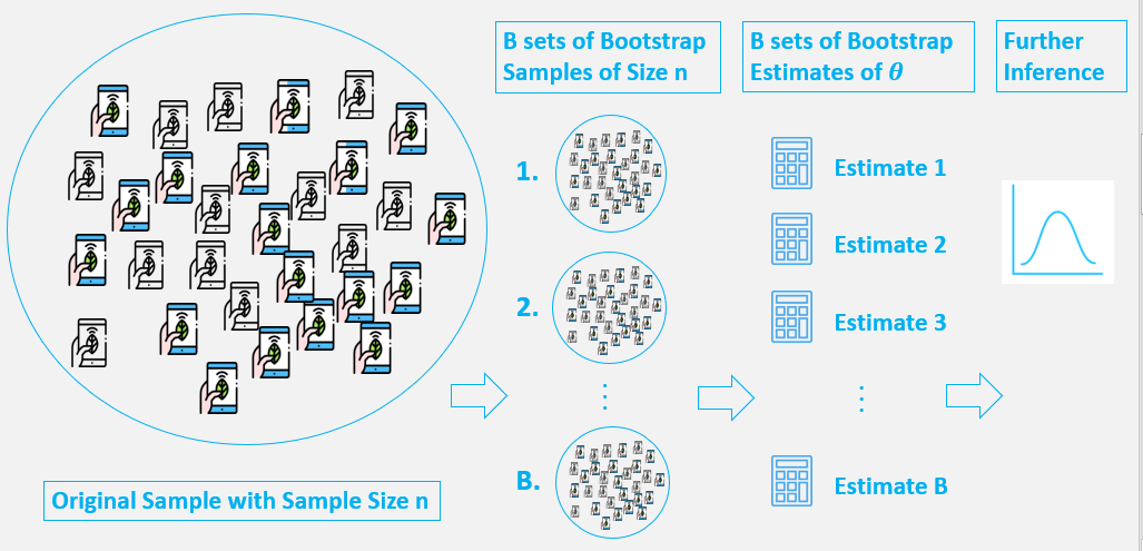
1. A sample from population with sample size north.
2. Draw a sample from the original sample data with replacement with size n, and replicate B times, each re-sampled sample is called a Bootstrap Sample, and in that location will totally B Bootstrap Samples.
3. Evaluate the statistic of θ for each Bootstrap Sample, and there will exist totally B estimates of θ.
4. Construct a sampling distribution with these B Bootstrap statistics and use it to make farther statistical inference, such as:

• Estimating the standard mistake of statistic for θ.
• Obtaining a Confidence Interval for θ.

We tin encounter we generate new data points by re-sampling from an existing sample, and brand inference only based on these new data points.

How and why does bootstrap work?

In this article, I will split up this big question into three parts:

1. What'southward the initial motivation that Efron introduced the bootstrap?
2. Why employ the simulation technique? In other word, how can I detect a estimated variance of statistic past resampling?
3. What's the chief idea that nosotros need to draw a sample from the original sample with replacement ?

I. Initial Motivation- The Reckoner's Standard Error

The core idea of bootstrap technique is for making sure kinds of statistical inference with the assist of modernistic reckoner power. When Efron introduced the method, it was particularly motivated by evaluating of the accuracy of an estimator in the field of statistic inference. Unremarkably, estimated standard error are an first step toward thinking critically about the accuracy statistical estimates.

Now, to illustrate how bootstrap works and how an reckoner'due south standard error plays an important office, permit'south get-go with a simple case.

Scenario Case

Imagine that you lot want to summarize how many times a twenty-four hour period practice students pick upwardly their smartphone in your lab with totally 100 students. Information technology's hard to summarize the number of pickups in whole lab like a census manner. Instead, you make a online survey which also provided the pickup-counting APP. In the side by side few days, you receive 30 students responses with their number of pickups in a given day. You calculated the mean of these xxx pickups and got an estimate for pickups is 228.06 times.

Codes for this case, just feel free to bank check out.

In statistic field, the procedure above is chosen a point guess. What we would like to know is the truthful number of pickups in whole lab. We don't have demography information, what we can exercise is just evaluate the population parameter through an calculator based on an observed sample, and then get an estimate as the evaluation of average smartphone usage in the lab.

• Estimator/Statistic: A rule for computing an estimate. In this case is Sample mean, always denoted every bit X̄.
• Population Parameter: Numeric summary nearly a population. In this example is the average fourth dimension of phone pickups per day in our lab, always denoted as μ.

One key question is — How accurate is this judge result?

Because of the sampling variability , it is about never that X̄ = μ occurs . Hence , too reporting the value of a point gauge, some indication virtually the precision should be given. The common measure of accuracy is the standard error of the gauge.

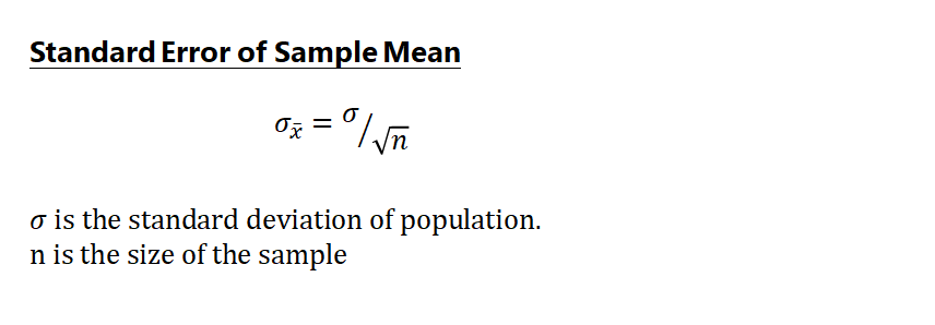
The Standard Error

The standard error of an estimator is it'south standard deviation. It tells us how far your sample estimate deviates from the actual parameter. If the standard mistake itself involves unknown parameters, we used the estimated standard fault by replacing the unknown parameters with an estimate of the parameters.

Let's have an example. In our case, our estimator is sample mean, and for sample mean(and most but one!), nosotros accept an simple formula to hands obtain it's standard error.

However, the standard departure of population σ is always unknown in existent world, and so the near common measurement is the estimated standard mistake, which utilise the sample standard departure S as a estimated standard deviation of the population:

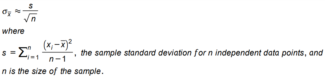
In our case, we have sample with thirty, and sample mean is 228.06, and the sample standard deviation is 166.97, and then our estimated standard error for our sample hateful is 166.97 / √30 = 30.48.

Standard Fault in Statistic Inference

Now we have got our estimated standard error. How can the standard fault be used in the statistic inference? Permit'due south use a unproblematic example to illustrate.

Roughly speaking, if a estimator has a normal distribution or a approximately a normal distributed, then we expect that our estimate to be less than i standard error away from its expectation about 68% of the time, and less than two standard errors away well-nigh 95% of the time.

In our case, call up that the sample we collected is 30 response sample, which is sufficiently large in thumb rule, the Cardinal Limit Theorem tells us the sampling distribution of X̄ is closely approximated to a normal distribution. Combining the estimated standard error that, we tin can get:

We tin can be reasonably confident that the true of μ, the the boilerplate times a day do students selection up their smartphone in our lab, lies within approximately 2 standard fault of X̄, which is (228.06 −2×thirty.48, 228.06+ii×30.48) = (167.one, 289.02).

The Ideal and Reality in Statistic World

We accept made our statistic inference. Even so, how this inference was going well is nether some rigorous assumptions.

Allow'south call up what supposition or classical theorem nosotros may have used then far:

• An standard mistake of our sample mean can exist hands estimated, which we take used standard deviation of sample as reckoner and a simple formula to obtain the estimated standard error.
• We assume we know or tin can estimate nearly the computer'southward population. In our case is the approximated normal distribution.

However, in our existent world, sometimes it'south hard to meet assumptions or theorem like higher up:

• It'due south hard to know the information about population, or it'due south distribution.
• The standard error of a estimate is hard to evaluate in general. Virtually of time, there is no a precise formula like standard mistake of sample mean. If now, nosotros want to make a inference for the median of the smart phone pickups, what's the standard error of sample median?

This is why the bootstrap comes in to address these kind of problems. When these assumptions are violated, or when no formula exists for estimating standard errors , bootstrap is the powerful choice.

Ii. Explanation about Bootstrap

To illustrate the main concepts, post-obit explanation volition evolve some mathematics definition and denotation, which are kind of informal in club to provide more than intuition and agreement.

1. Initial Scenario

Assume we want to estimate the standard error of our statistic to make an inference most population parameter, such as for constructing the respective confidence interval (just like what we take washed before!). And:

• We don't know annihilation virtually population.
• There is no precise formula for estimating the standard error of statistic.

Let X1, X2, … , Xn be a random sample from a population P with distribution function F . And permit M= thousand(X1, X2, …, Xn), be our statistic for parameter of interest, significant that the statistics a function of sample data X1, X2, …, Xn. What we want to know is the variance of M, denoted every bit Var(M).

• First, since we don't know anything about population, we can't determine the value of Var(1000) that requires known parameter of population, and then we need to estimate Var(M) with a estimated standard fault , denoted as EST_Var(M). (Call up the estimated standard error of sample mean?)
• Second, in real world nosotros always don't have a simple formula for evaluating the EST_Var(M) other than the sample hateful'southward.

It leads us demand to approximate the EST_Var(M). How? Earlier answer this , allow's introduce an common practical manner is simulation, assume we know P.

2. Simulation

Allow's talk nigh the idea of simulation. It's useful for obtaining information near a statistic's sampling distribution with the help of computers. Only it has an important supposition — Assume we know the population P.

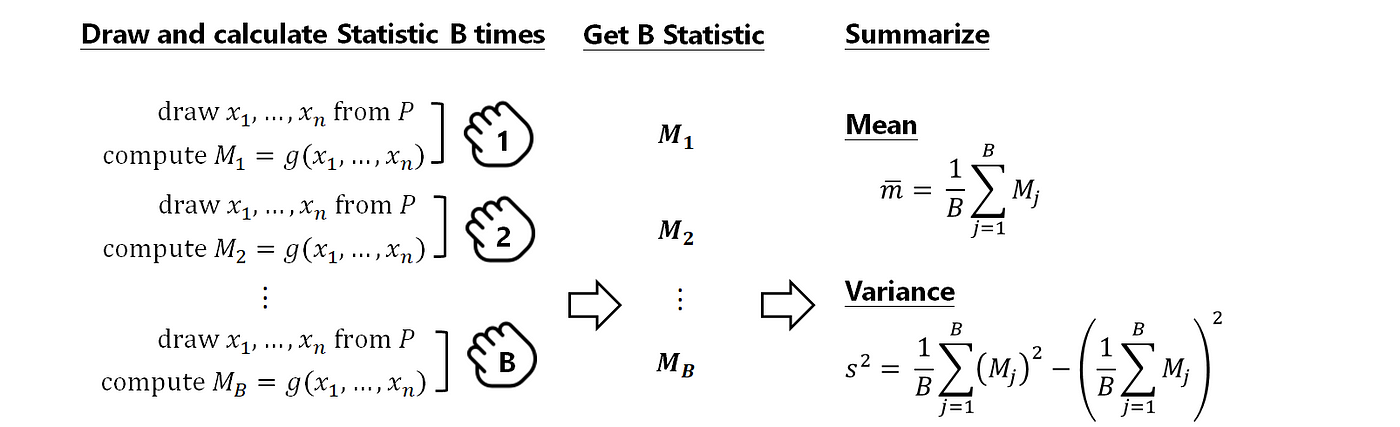
Now let X1, X2, … , Xn be a random sample from a population and assume M= g(X1, X2, …, Xn) is the statistic of interest, nosotros could approximate mean and variance of statistic M by simulation as follows:

1. Draw random sample with size n from P.
2. Compute statistic for the sample.
3. Replicate B times for procedure 1. and 2 and get B statistics.
4. Get the mean and variance for these B statistics.

Why does this simulation works? Since by a classical theorem, the Police force of Big Numbers:

• The mean of these B statistic converges to the true mean of statistic Chiliad as B → ∞.

And by Law of Large Numbers and several theorem related to Convergence in Probability:

• The sample variance of these B statistic converges to the true variance of statistic Yard equally B → ∞.

With the help of computer, we can make B as large as we similar to estimate to the sampling distribution of statistic Yard.

Following is the example Python codes for simulation in the previous phone-picks example. I utilize B=100000, and the false mean and standard fault for sample mean is very close to the theoretical results in the last 2 cells. Feel gratuitous to bank check out.

Case codes for simulation applied with the previous phone-picks case start from cell [10].

3. The Empirical Distribution Part and Plug-in Principle

We accept learned the thought of simulation. At present, can nosotros approximate the EST_Var(One thousand) by simulation? Unfortunately, to practice the simulation to a higher place, we need to know the information nearly population P. The truth is that we don't know anything about the P. For addressing this result, ane of most important component in bootstrap Method is adopted:

Using Empirical distribution office to guess the distribution function of population, and applying Plug-in Principle to go an approximate for Var(Grand) — the Plug-in computer.

(1) Empirical Distribution Function

The idea of Empirical distribution function (EDF) is building an distribution function (CDF) from an existing information set. The EDF ordinarily approximates the CDF quite well, especially for large sample size. In fact, information technology is a common, useful method for estimating a CDF of a random variable in pratical.

The EDF is a discrete distribution that gives equal weight to each data point (i.e., it assigns probability i/ n to each of the original due north observations), and class a cumulative distribution role that is a step role that jumps up past ane/northward at each of the due north data points.

(2) Statistical Functional

Bootstrap employ the EDF equally an estimator for CDF of population. Withal, we know the EDF is a type of cumulative distribution function(CDF). To apply the EDF as an estimator for our statistic M, we need to brand the form of Thou as a office of CDF type, even the parameter of interest as well to have the some base line. To do this, a common way is the concept called Statistical Functional. Roughly speaking, a statistical functional is whatever office of a distribution office. Let's have an case:

Suppose nosotros are interested in parameters of population. In statistic field , in that location is always a situation where parameters of involvement is a function of the distribution office, these are called statistical functionals. Following listing that population hateful East(X) is a statistical functional:

From above nosotros can meet the mean of population E(X) can as well be expressed as a grade of CDF of population F — this is a statistical functional. Of class, this expression can be applied to any function other than mean, such equally variance.

Statistical functional can be viewed as quantity describing the features of the population. The mean, variance, median, quantiles of F are features of population. Thus, using statistical functional, we have a more than rigorous way to define the concepts of population parameters. Therefore, we can say, our statistic M can be : M=1000(F), with the population CDF F.

(three) Plug-in Principle = EDF + Statistical Functional

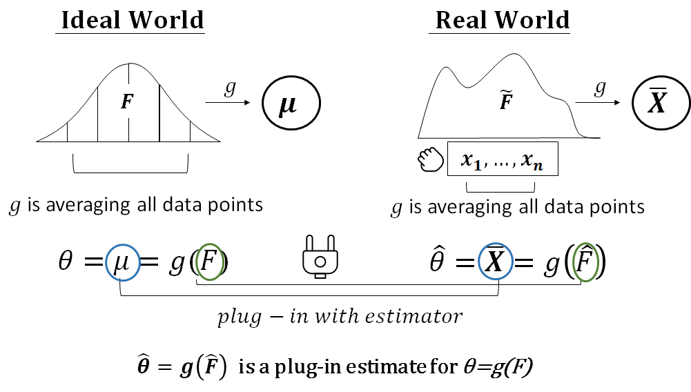
Nosotros have made our statistic is M= thou(X1, X2, …, Xn)=k(F) be a statistical functional course. However, we don't know F. And then we take to "plug-in" a calculator for F, "into" our M=1000(F), in order to make this Grand can be evaluate.

It is called plug-in principle. More often than not speaking, the plug-in principle is a method of interpretation of statistical functionals from a population distribution by evaluating the aforementioned functionals, but with the empirical distribution which is based on the sample. This estimation is chosen a plug-in estimate for the population parameter of involvement. For example, a median of a population distribution can be approximated by the median of the empirical distribution of a sample. The empirical distribution here, is class just past the sample because we don't know population. Put it simply:

• If our parameter of interest , say θ, has the statistical function form θ=1000(F), which F is population CDF.
• The plug-in calculator for θ=g(F), is defined to be θ_hat=thousand(F_hat):

• From above formula we can see nosotros "plug in" the θ_hat and F_hat for the unknown θ and F. F_hat here, is purely estimated by sample data.
• Note that both of the θ and θ_hat are determined past the aforementioned role yard(.).

Permit'due south accept an mean case as follows, we can see one thousand(.) for mean is — averaging all information points, and information technology is also applied for sample mean. F_hat here, is form by sample as an estimator of F. We say the sample hateful is a plug-in estimator of the population mean.(A more clear outcome will be provided soon.)

So, what is the F_hat? Remember bootstrap use Empirical distribution function(EDF) as an reckoner of CDF of population? In fact, EDF is likewise a common estimator that be widely used in plug-in principle for F_hat.

Let's have a look what does our estimator 1000= g(X1, X2, …, Xn)=g(F) will look like if we plug-in with EDF into information technology.

• Let Statistic of interest be M=g(X1, X2, …, Xn)= g(F) from a population CDF F.
• We don't know F, and then we build a Plug-in estimator for M, M becomes M_hat= g(F_hat). Permit's rewrite M_hat every bit follows:

We know EDF is a discrete distribution that with probability mass office PMF assigns probability 1/ n to each of the north observations, and so co-ordinate this, M_hat becomes:

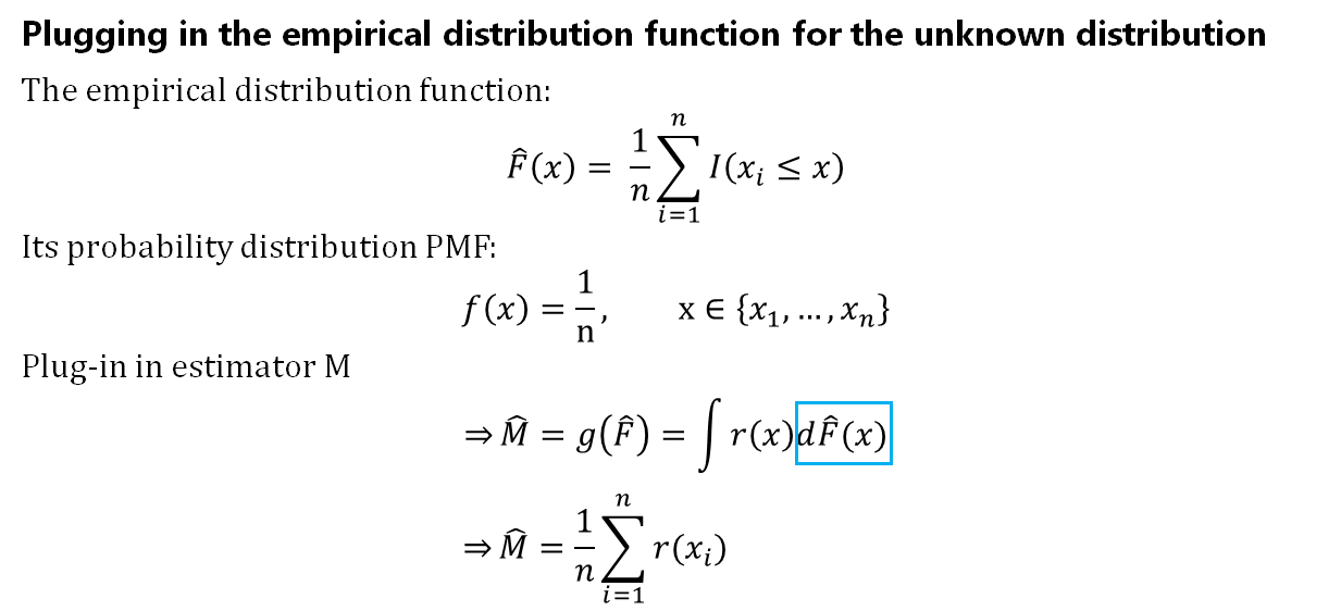
Co-ordinate this, for our mean example, nosotros can find the plug-in estimator for mean μ is just the sample mean:

Hence, we through Plug-in Principle, to brand an estimate for M=g(F), say M_hat=g(F_hat). And remember that, what we want to find out is Var(M), and nosotros approximate Var(One thousand) by Var(M_hat). Just in general case, there is no precise formula for Var(M_hat) other than sample mean! It leads u.s.a. to apply a simulation.

(iv) Bootstrap Variance Estimation

It's nearly the last footstep! Let'south refresh the whole procedure with the Plug-in Principle concept.

Our goal is to estimate the variance of our estimator M, which is Var(Yard). The Bootstrap principle is as follows:

1. Nosotros don't know the population P with CDF denoted as F, then bootstrap use Empirical distribution function(EDF) every bit estimate of F.
2. Using our existing sample data to form a EDF as a estimated population.
3. Applied the Plug-in Principle to brand Yard=g(F) can be evaluate with EDF. Hence, One thousand=m(F) becomes M_hat= g(F_hat), it's the plugged-in estimator with EDF — F_hat.
4. Take simulation to approximate to the Var(M_hat).

Remember that to practise the original version of simulation, we demand to describe a sample information from population, obtain a statistic 1000=yard(F) from information technology, and replicate the procedure B times, and then go variance of these B statistic to approximate the true variance of statistic.

Therefore, to do simulation in step iv, we demand to:

1. Draw a sample data from EDF.
2. Obtain a plug-in statistic M_hat= thou(F_hat).
3. Replicate the two procedure B times.
4. Get the variance of these B statistic, to estimate the true variance of plug-in statistic.(It'southward an easily confused office.)

What'south the simulation? In fact, it is the bootstrap sampling procedure that we mentioned in the outset of this commodity!

Two questions hither(I promise these are terminal two!):

1. How does depict from EDF look like in step one?
2. How does this simulation work?

How does describe from EDF look like?

Nosotros know EDF builds an CDF from existing sample data X1, …, Xn, and by definition information technology puts mass 1/n at each sample data point. Therefore, drawing an random sample from an EDF, tin exist seen as cartoon due north observations, with replacement, from our existing sample data X1, …, Xn. And then that'southward why the bootstrap sample is sampled with replacement as shown before.

How does simulation work?

The variance of plug-in estimator M_hat=g(F_hat) is what the bootstrap simulation want to simulate. At the beginning of simulation, we draw observations with replacement from our existing sample data X1, …, Xn. Let'south announce these re-sampled data X1* , …, Xn*. Now, let's compare bootstrap simulation with our original simulation version again .

Original simulation process for Var(1000=grand(F)):

                      Original Simulation Version- Approximate EST_Var(M|F) with known F                    Let X1, X2, … , Xn exist a random sample from a population            P            and assume            Thousand= one thousand(X1, X2, …, Xn) is the statistic of interest, we could approximate variance of statistic            Chiliad            past simulation as follows:          1. Draw random sample with size n from P.
2. Compute statistic for the sample.
3. Replicate B times for procedure i. and 2 and become B statistics.
iv. Become the variance for these B statistics.        

Same with previous Simulation part for simulating Var(M).

Bootstrap Simulation for Var(M_hat=yard(F_hat))

                      Bootstrap Simulation Version- Guess Var(M_hat|F_hat) with EDF                    Now let X1, X2, … , Xn be a random sample from a population            P with CDF F,            and assume            M= grand(X1, X2, …, Xn ;F) is the statistic of interest. But nosotros don't know F, then we:          1.Form a EDF from the existing sample data by describe observations with replacement from our existing sample information X1, …, Xn. These are denote equally X1*, X2*, …, Xn*. We call this is a bootstrap sample.          ii.Compute statistic            M_hat= g(X1*, X2*, …, Xn* ;F_hat) for the bootstrap sample.          3. Replicate B times for steps two and iii, and get B statistics M_hat.          4. Become the variance for these B statistics to approximate the            Var(M_hat).        

Simulating for Var(M_hat).

Would you feel familiar with processes above? In fact, it'due south the same procedure with bootstrap sampling method we take mentioned earlier!

III. What Does the Bootstrap Piece of work?

Finally, let's check out how does our simulation will work. What we will get the approximation from this bootstrap simulation is for Var(M_hat), but what we really business concern is whether Var(M_hat) can approximate to Var(M). Then ii question here:

1. Will bootstrap variance simulation consequence, which is Due south², can judge well for Var(M_hat)?
2. Can Var(M_hat) tin approximate to Var(G)?

To answer this ,permit's apply a diagram to illustrate the both types simulation mistake:

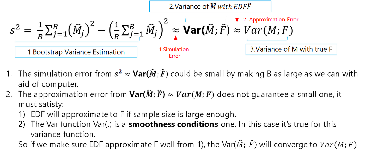
1. From bootstrap variance estimation, nosotros will go an estimate for Var(M_hat) — the plug-in estimate for Var(Thousand). And the Constabulary of Large Number tell us, if our simulation times B is large plenty, the bootstrap variance interpretation South², is a good guess for Var(M_hat). Fortunately, nosotros can get a larger B as we similar with aid of a computer. So this simulation fault can be small.
2. The Variance of M_hat, is the plug-in estimate for variance of One thousand from true F. Is the Var(M_hat; F_hat) a skillful computer for Var(M; F)? In other words, does a plug-in estimator approximate well to the reckoner of interest ? That'due south the key point what we really concern. In fact, the topic of asymptotic properties for plug-in estimators is classified in loftier level mathematical statistic. But let's explain the main issues and ideas.

• Get-go, We know the empirical distribution will converges to true distribution office well if sample size is large, say F_hat → F.
• Second, if F_hat → F, and if it'south corresponding statistical function 1000(.) is a smoothness weather condition, and then g(F_hat) → g(F). In our instance, the statistical function yard(.) is Variance, which satisfy the required continuity atmospheric condition. Therefore, that explains why the bootstrap variance is a good estimate of the true variance of the calculator Yard.

By and large, the smoothness conditions on some functionals is hard to verify. Fortunately, most mutual statistical functions like mean, variance or moments satisfy the required continuity weather condition. It provides that bootstrapping works. And of course, make the original sample size not likewise pocket-sized as nosotros can.

Below is my Bootstrap sample code for pickup case, savage costless to bank check out.

Bootstrap Epitomize

Let'southward epitomize the primary ideas of bootstrap with following diagram!

Source: https://towardsdatascience.com/an-introduction-to-the-bootstrap-method-58bcb51b4d60

Share this post